Einführung

An diesem Kurstag möchten wir uns mit der Auswertung von Daten aus einer RNA Sequenzierung (RNA-seq) beschäftigen.

RNA-seq Daten sind so genannte high-throughput count Daten, in denen wir in vielen parallelen Analysen zählen, wieviele reads pro Gen oder Transkript im Sample detektiert wurden.

Sequenzierungsbibliothek: alle Nukleotide eines Samples, welche den Input für unser Sequenzierungsexperiment darstellen
Fragmente: Da der aktuelle technologische Goldstandard (Illumina Sequenzierung) nur Nukleotide von wenigen hundert Basenpaaren analysieren kann, müssen diese vor der Analyse fragmentiert werden
Read: Sequenz welche von einem Fragment erhoben wird. Ca. 150 bp bei Illumina. Bei RNA-seq und doppelsträngiger cDNA bezieht sich dies auf jeweils einen Strang

Zeitliche Abfolge: 1. Sequenzierung > 2. Counting

Benötigte Pakete

pasilla: Paket, welches die Bespieldaten enthält
DESeq2: DAS Paket für die Analyse von RNA-seq Daten
pheatmap: Paket zur Erstellung von Heatmaps (sehr gute Alternative ComplexHeatmap Paket)
broom: Paket für Ergebnisstabellen

Beispieldatensatz

Unseren Bespieldatensatz beziehen wir aus dem Paket pasilla

fn <- system.file("extdata", "pasilla_gene_counts.tsv",
                  package = "pasilla", mustWork = TRUE)

counts <- as.matrix(read.csv(fn, sep = "\t", row.names = "gene_id"))

Sequenzierungsdaten sollten als Matrix gespeichert sein und nicht als Dataframe bzw. Tibble!

dim(counts)

## [1] 14599     7

counts[1:3,]

##             untreated1 untreated2 untreated3 untreated4 treated1 treated2
## FBgn0000003          0          0          0          0        0        0
## FBgn0000008         92        161         76         70      140       88
## FBgn0000014          5          1          0          0        4        0
##             treated3
## FBgn0000003        1
## FBgn0000008       70
## FBgn0000014        0

Diese Matrix wird auch count table genannt. Wir haben Countdaten zu 14,599 Genen von 7 Samples. Hierbei handelt es sich um die “raw” Counts.

Herausforderungen der Datenanalyse

großer Wertebereich (0-Millionen)
Die nicht-negativen Count Daten (Integers) folgen keine symmetrischen Verteilung und damit keiner! Normalverteilung

plot(density(counts), xlim=c(0,10000), xlab = "Counts", main = "", bty="none")

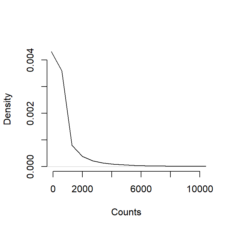
Im Count Daten zwischen Samples zu vergleichen bedarf es einer Normalisierung. Faktoren sind hier u.a. die Sequenzierungsbibliothek, Sequenzierungstiefe, Genlänge, GC content.

Beispieldatensatz - Informationen zu Samples und zum Experiment

RNAi Knockdown Experiment des Splicingfaktors pasilla in D. melanogaster. Zwei Konditionen: treated und untreated. Den Annotationfile laden wir mit:

annotationFile <- system.file("extdata",
  "pasilla_sample_annotation.csv",
  package = "pasilla", mustWork = TRUE)
pasillaSampleAnno <- readr::read_csv(annotationFile)

pasillaSampleAnno <- mutate(pasillaSampleAnno,
condition <- factor(condition, levels = c("untreated", "treated")),
type <- factor(sub("-.*", "", type), levels = c("single", "paired")))

pasillaSampleAnno

## # A tibble: 7 x 8
##   file  condition type  `number of lane~ `total number o~ `exon counts`
##   <chr> <chr>     <chr>            <dbl> <chr>                    <dbl>
## 1 trea~ treated   sing~                5 35158667              15679615
## 2 trea~ treated   pair~                2 12242535 (x2)         15620018
## 3 trea~ treated   pair~                2 12443664 (x2)         12733865
## 4 untr~ untreated sing~                2 17812866              14924838
## 5 untr~ untreated sing~                6 34284521              20764558
## 6 untr~ untreated pair~                2 10542625 (x2)         10283129
## 7 untr~ untreated pair~                2 12214974 (x2)         11653031
## # ... with 2 more variables: `condition <- factor(condition, levels =
## #   c("untreated", "treated"))` <fct>, `type <- factor(sub("-.*", "", type),
## #   levels = c("single", "paired"))` <fct>

with(pasillaSampleAnno,
       table(condition, type))

##            type
## condition   paired-end single-read
##   treated            2           1
##   untreated          2           2

DESeq2 - DAS R Paket für die Analyse von RNA-seq Daten

Das DESeq2 gehört zu den weltweit meist genutzen Pakten zur Analyse von RNA-seq Datensätzen.

Bevor wir mit der Analyse starten können, gilt es aus der Matrix counts und dem Dataframe der die Sampleinfo beschreibt pasillaSampleAnno ein sogenanntes DESeqDataSet zu erstellen:

mt <- match(colnames(counts), sub("fb$", "", pasillaSampleAnno$file))
stopifnot(!any(is.na(mt)))

pasilla <- DESeqDataSetFromMatrix(
  countData = counts,
  colData   = pasillaSampleAnno[mt, ],
  design    = ~ condition)

pasilla

## class: DESeqDataSet 
## dim: 14599 7 
## metadata(1): version
## assays(1): counts
## rownames(14599): FBgn0000003 FBgn0000008 ... FBgn0261574 FBgn0261575
## rowData names(0):
## colnames(7): untreated1 untreated2 ... treated2 treated3
## colData names(8): file condition ... condition <- factor(condition,
##   levels = c("untreated", "treated")) type <- factor(sub("-.*", "",
##   type), levels = c("single", "paired"))

Durchführung der differentiellen Expressionsanalyse

Ziel: Gene identifizieren, die zwischen treated und untreated Samples unterschiedlich sind. Wir wenden hier einen Hypothesentest an, der mit dem t-Test mathematisch verwandt ist.

pasilla <- DESeq(pasilla)

pasilla

## class: DESeqDataSet 
## dim: 14599 7 
## metadata(1): version
## assays(4): counts mu H cooks
## rownames(14599): FBgn0000003 FBgn0000008 ... FBgn0261574 FBgn0261575
## rowData names(22): baseMean baseVar ... deviance maxCooks
## colnames(7): untreated1 untreated2 ... treated2 treated3
## colData names(9): file condition ... type <- factor(sub("-.*", "",
##   type), levels = c("single", "paired")) sizeFactor

Results

res <- results(pasilla)
res[order(res$padj), ] %>% head

## log2 fold change (MLE): condition untreated vs treated 
## Wald test p-value: condition untreated vs treated 
## DataFrame with 6 rows and 6 columns
##                     baseMean    log2FoldChange              lfcSE
##                    <numeric>         <numeric>          <numeric>
## FBgn0039155 730.595806139728    4.619013535193  0.168706755496974
## FBgn0025111 1501.41051323996 -2.89986418283187  0.126920467532813
## FBgn0029167 3706.11653071978  2.19700028710382 0.0969888689039936
## FBgn0003360 4343.03539692487  3.17967242210135  0.143526226262858
## FBgn0035085 638.232608936723  2.56041205175815  0.137295199514033
## FBgn0039827 261.916235943103  4.16251610026134  0.232588756794067
##                          stat                pvalue                  padj
##                     <numeric>             <numeric>             <numeric>
## FBgn0039155  27.3789482915866 4.88534640286228e-165 4.06607381110228e-161
## FBgn0025111 -22.8478844996546 1.53390416993678e-115 6.38334220319191e-112
## FBgn0029167  22.6520869036895 1.33057630038134e-113 3.69146218269131e-110
## FBgn0003360  22.1539470861445 9.55682092175738e-109 1.98853551329467e-105
## FBgn0035085  18.6489553955341  1.28768628708899e-77  2.14348259348833e-74
## FBgn0039827   17.896463086334  1.25652932702639e-71  1.74301559814011e-68

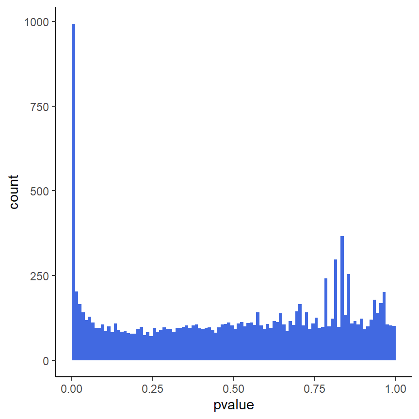
Im folgenden möchten wir die Results der differentiellen Expressionsanalyse mithilfe von Visualisierungen explorieren.

Histogramm der p-Werte

ggplot(as(res, "data.frame"), aes(x = pvalue)) +
  geom_histogram(binwidth = 0.01, fill = "Royalblue", boundary = 0) +
    theme_classic()

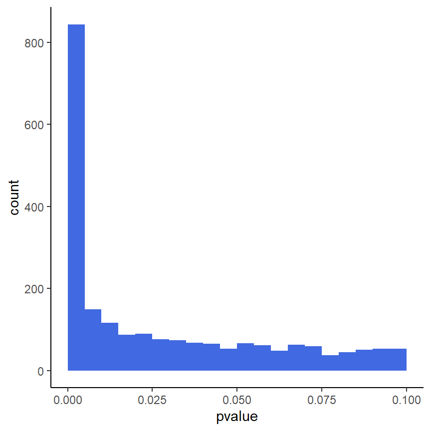
ggplot(as(res, "data.frame"), aes(x = pvalue)) +
  geom_histogram(binwidth = 0.005, fill = "Royalblue", boundary = 0) +
    xlim(c(0,0.1)) +
    theme_classic()

MA plot

Fold change (M-value) vs. average counts (A-value)

plotMA(pasilla, ylim = c( -2, 2))

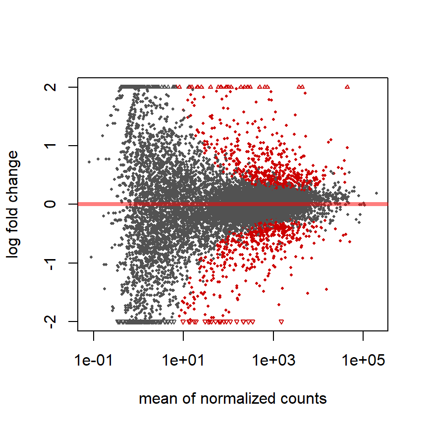
Roten Punkte = adjustierter P-Wert < 0.1

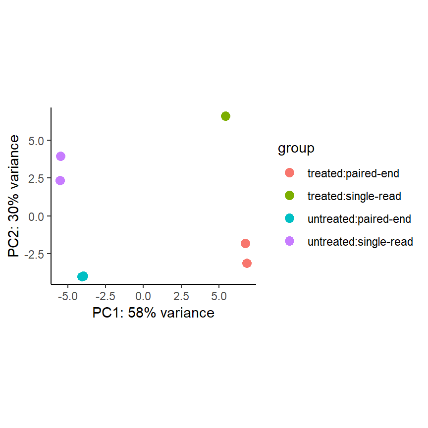
PCA plot

Die Principle Component Analysis (PCA) ist eine Methodik zur Dimensionsreduktion. Hierbei werden für jeden Sample die Infos zu allen 14,599 Genen auf zwei Dimensionen (x- und y-Achse) reduziert. Ein Sample ist ein Punkt auf dem Plot.

pas_rlog <- rlogTransformation(pasilla)
plotPCA(pas_rlog, intgroup=c("condition", "type")) + 
    coord_fixed() +
    theme_classic()

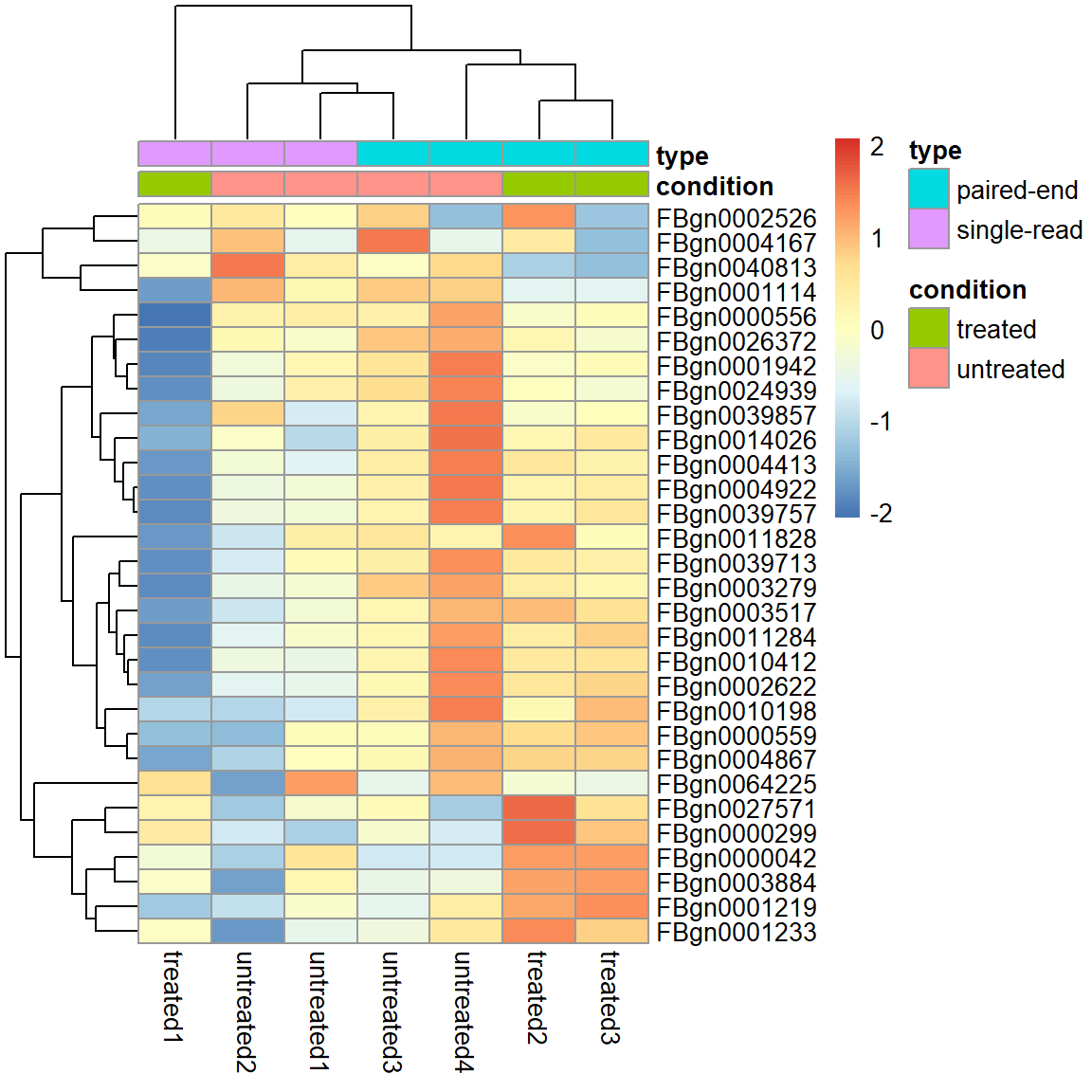
Heatmap

Eine Heatmap aller Gene darzustellen macht keinen Sinn. Es gilt Filterkriterien zu definieren.

Filter 1) Top 30 most expressed genes.

select <- order(rowMeans(assay(pas_rlog)), decreasing = TRUE)[1:30]

pheatmap( assay(pas_rlog)[select, ],
     scale = "row",
     annotation_col = as.data.frame(
        colData(pas_rlog)[, c("condition", "type")] ))

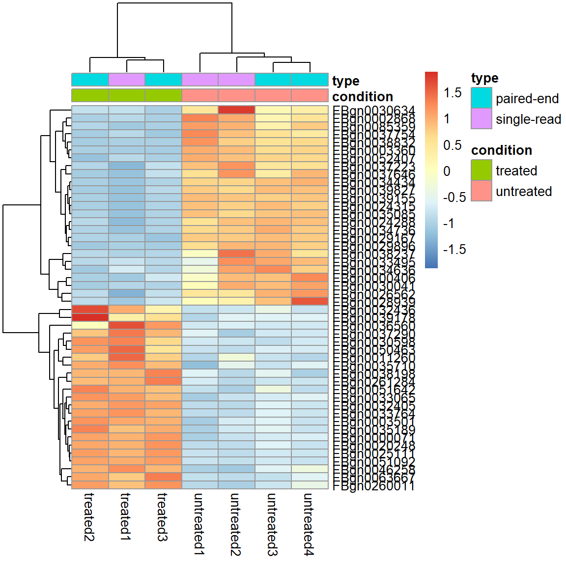
Filter 2) Adjusted p-Value < 0.01 und absolute log2 Fold Change > 2

select2 <- (res$padj<0.01 & abs(res$log2FoldChange)>2)*1

pheatmap( assay(pas_rlog)[select2 %in% 1, ],
     scale = "row",
     annotation_col = as.data.frame(
        colData(pas_rlog)[, c("condition", "type")] ))

Einführung in R Programming

Tag 5 - RNA-seq Analyse

Kursmaterial zur RNA-seq Analyse