Einführung in R Programming
Tag 2 - Datentransformation und Plotting
Andreas Mock
Ablauf - Tag 2
- Datentransformation mit
dplyr
- Datenvisualisierung mit
ggplot2
Erweiterung der R Objektfamilie
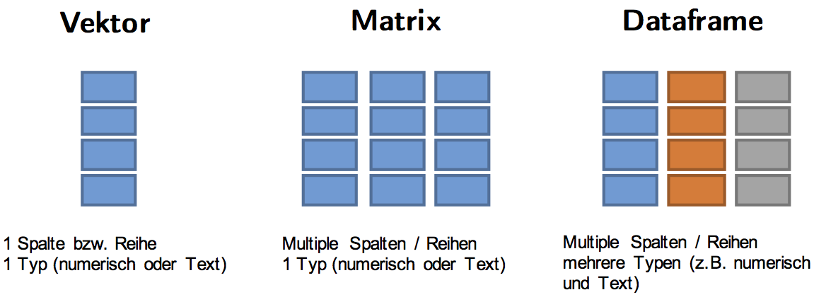
- Faktor: spezielle Unterform eines Vektors für kategoriale Variablen. Ein Faktor fasst die Kategorien (= Levels) zusammen.
# Vektor
head(hnscc$grade)
## [1] "G3" "G2" "G2" "G2" "G2" "G1"
# Faktor
head(as.factor(hnscc$grade))
## [1] G3 G2 G2 G2 G2 G1
## Levels: G1 G2 G3 G4 GX
Tibbles - moderne Dataframes
## [1] "tbl_df" "tbl" "data.frame"
Der hnscc Datensatz ist eigentlich streng genommen kein Dataframe, sondern ein sogenannter Tibble, die moderne Weiterentwicklung eines R Dataframes.
## # A tibble: 279 x 11
##    id            age alcohol days_to_death gender neoplasm_site grade pack_years
##    <chr>       <int> <chr>           <int> <chr>  <chr>         <chr>      <dbl>
##  1 TCGA-BA-40~    69 YES               461 MALE   Oral Tongue   G3            51
##  2 TCGA-BA-40~    39 YES               415 MALE   Larynx        G2            30
##  3 TCGA-BA-40~    45 YES              1134 FEMALE Base of Tong~ G2            30
##  4 TCGA-BA-40~    83 NO                276 MALE   Larynx        G2            75
##  5 TCGA-BA-51~    47 YES               248 MALE   Floor of Mou~ G2            60
##  6 TCGA-BA-51~    72 YES               190 MALE   Buccal Mucosa G1            20
##  7 TCGA-BA-51~    56 YES               845 MALE   Alveolar Rid~ G2            NA
##  8 TCGA-BA-51~    51 YES              1761 MALE   Tonsil        G2            NA
##  9 TCGA-BA-55~    54 YES               186 MALE   Larynx        G2            62
## 10 TCGA-BA-55~    58 YES               179 FEMALE Floor of Mou~ G3            60
## # ... with 269 more rows, and 3 more variables: tabacco_group <chr>,
## #   tumor_stage <chr>, vital_status <chr>
Tibbles - moderne Datenframes
Im Vergleich dazu der Output eines “normalen” Dataframes. In Übung 3 werdet ihr die Unterschiede herausarbeiten.
head(as.data.frame(hnscc))
##             id age alcohol days_to_death gender  neoplasm_site grade pack_years
## 1 TCGA-BA-4074  69     YES           461   MALE    Oral Tongue    G3         51
## 2 TCGA-BA-4076  39     YES           415   MALE         Larynx    G2         30
## 3 TCGA-BA-4077  45     YES          1134 FEMALE Base of Tongue    G2         30
## 4 TCGA-BA-4078  83      NO           276   MALE         Larynx    G2         75
## 5 TCGA-BA-5149  47     YES           248   MALE Floor of Mouth    G2         60
## 6 TCGA-BA-5151  72     YES           190   MALE  Buccal Mucosa    G1         20
##                                 tabacco_group tumor_stage vital_status
## 1                              Current smoker   Stage IVA     DECEASED
## 2                              Current smoker        <NA>     DECEASED
## 3 Current reformed smoker for < or = 15 years   Stage IVA     DECEASED
## 4 Current reformed smoker for < or = 15 years        <NA>     DECEASED
## 5                              Current smoker   Stage IVA       LIVING
## 6      Current reformed smoker for > 15 years   Stage IVA       LIVING
Zeilen filtern mit filter()
Die Funktion filter() ermöglicht es uns ein Subset aus den Zeilen auszuwählen. Das erste Argument ist das Objekt, die weiteren Argumente sind die Spalten, wonach wir filtern möchten.
young <- filter(hnscc, age<50)

young
## # A tibble: 42 x 11
##    id            age alcohol days_to_death gender neoplasm_site grade pack_years
##    <chr>       <int> <chr>           <int> <chr>  <chr>         <chr>      <dbl>
##  1 TCGA-BA-40~    39 YES               415 MALE   Larynx        G2            30
##  2 TCGA-BA-40~    45 YES              1134 FEMALE Base of Tong~ G2            30
##  3 TCGA-BA-51~    47 YES               248 MALE   Floor of Mou~ G2            60
##  4 TCGA-BA-55~    41 YES               242 FEMALE Oral Tongue   G2            NA
##  5 TCGA-BA-68~    47 YES               395 MALE   Floor of Mou~ G2            40
##  6 TCGA-BA-68~    28 YES               113 MALE   Oral Tongue   G2             1
##  7 TCGA-BB-42~    48 NO               2891 MALE   Tonsil        G3            NA
##  8 TCGA-CN-47~    19 NO                240 MALE   Oral Tongue   G2            NA
##  9 TCGA-CN-47~    48 YES               397 FEMALE Oral Tongue   G3            20
## 10 TCGA-CN-53~    48 YES               252 MALE   Larynx        G3            15
## # ... with 32 more rows, and 3 more variables: tabacco_group <chr>,
## #   tumor_stage <chr>, vital_status <chr>
larynx <- filter(hnscc, neoplasm_site=="Larynx")

larynx
## # A tibble: 72 x 11
##    id            age alcohol days_to_death gender neoplasm_site grade pack_years
##    <chr>       <int> <chr>           <int> <chr>  <chr>         <chr>      <dbl>
##  1 TCGA-BA-40~    39 YES               415 MALE   Larynx        G2            30
##  2 TCGA-BA-40~    83 NO                276 MALE   Larynx        G2            75
##  3 TCGA-BA-55~    54 YES               186 MALE   Larynx        G2            62
##  4 TCGA-BA-68~    53 YES               152 MALE   Larynx        G2            60
##  5 TCGA-BA-68~    62 YES               244 MALE   Larynx        G2            46
##  6 TCGA-BA-68~    60 YES               450 FEMALE Larynx        G2            40
##  7 TCGA-BB-42~    68 YES               186 MALE   Larynx        G3            60
##  8 TCGA-CN-47~    67 YES               412 MALE   Larynx        G2            NA
##  9 TCGA-CN-47~    56 YES               194 MALE   Larynx        G2            80
## 10 TCGA-CN-47~    52 YES               369 MALE   Larynx        G3           120
## # ... with 62 more rows, and 3 more variables: tabacco_group <chr>,
## #   tumor_stage <chr>, vital_status <chr>
Logische Operatoren
Die doppelten Gleichheitszeichen entsprechen der Frage: Ist der Eintrag in neoplasm_site = "Larynx". Das Resultat der Frage ist ein Vektor mit den Informationen TRUE oder FALSE pro Eintrag eines Vektors.
table(hnscc$neoplasm_site=="Larynx")
##
## FALSE  TRUE
##   207    72
Die Notation um alle Sites außer Larynx zu filtern ist, ein Ausrufezeichen vor den Ausdruck zu setzen:
filter(hnscc, !neoplasm_site=="Larynx")
Mehrere Sites können wie folgt ausgewählt werden:
filter(hnscc, neoplasm_site %in% c("Tonsil", "Oral Tongue", "Hard Palate"))
Im Filterprozess können Informationen aus beliebig vielen Spalten miteinander kombiniert werden.
young_larynx <- filter(hnscc, age<50, neoplasm_site=="Larynx")

young_larynx
## # A tibble: 8 x 11
##   id             age alcohol days_to_death gender neoplasm_site grade pack_years
##   <chr>        <int> <chr>           <int> <chr>  <chr>         <chr>      <dbl>
## 1 TCGA-BA-4076    39 YES               415 MALE   Larynx        G2            30
## 2 TCGA-CN-5363    48 YES               252 MALE   Larynx        G3            15
## 3 TCGA-CN-6022    49 <NA>              201 MALE   Larynx        G3            NA
## 4 TCGA-CN-6988    47 YES                42 MALE   Larynx        G3            40
## 5 TCGA-CR-7371    45 NO                 93 FEMALE Larynx        G2            60
## 6 TCGA-CV-7433    49 NO                600 MALE   Larynx        G3            16
## 7 TCGA-CV-7440    38 NO                669 MALE   Larynx        GX            21
## 8 TCGA-F7-7848    47 YES                35 MALE   Larynx        G2            20
## # ... with 3 more variables: tabacco_group <chr>, tumor_stage <chr>,
## #   vital_status <chr>
Zeilen sortieren mit arrange()
Die Funktion arrange() sortiert Zeilen nach Spalteninformationen.
## # A tibble: 279 x 11
##    id            age alcohol days_to_death gender neoplasm_site grade pack_years
##    <chr>       <int> <chr>           <int> <chr>  <chr>         <chr>      <dbl>
##  1 TCGA-BA-51~    72 YES               190 MALE   Buccal Mucosa G1            20
##  2 TCGA-BA-55~    65 YES              1635 MALE   Hard Palate   G1            NA
##  3 TCGA-BA-72~    61 YES               236 MALE   Oral Tongue   G1            46
##  4 TCGA-CN-53~    55 YES               413 FEMALE Floor of Mou~ G1            60
##  5 TCGA-CR-73~    52 YES              1440 MALE   Oral Cavity   G1            45
##  6 TCGA-CR-73~    45 YES               759 MALE   Oral Tongue   G1            NA
##  7 TCGA-CR-73~    69 YES              1430 MALE   Oral Cavity   G1            54
##  8 TCGA-CR-73~    36 YES               913 FEMALE Oral Tongue   G1            NA
##  9 TCGA-CR-73~    67 NO                946 FEMALE Oral Tongue   G1            30
## 10 TCGA-CV-64~    62 NO                743 MALE   Oral Tongue   G1            NA
## # ... with 269 more rows, and 3 more variables: tabacco_group <chr>,
## #   tumor_stage <chr>, vital_status <chr>
Hierbei kann wie auch beim Filtern eine Sortierung in mehreren Schritten erfolgen.
arrange(hnscc, age, grade)
## # A tibble: 279 x 11
##    id            age alcohol days_to_death gender neoplasm_site grade pack_years
##    <chr>       <int> <chr>           <int> <chr>  <chr>         <chr>      <dbl>
##  1 TCGA-CN-47~    19 NO                240 MALE   Oral Tongue   G2            NA
##  2 TCGA-CR-73~    26 YES               908 MALE   Oral Tongue   G2            NA
##  3 TCGA-CV-59~    26 YES              1315 MALE   Oral Tongue   G2            NA
##  4 TCGA-BA-68~    28 YES               113 MALE   Oral Tongue   G2             1
##  5 TCGA-CV-74~    29 <NA>              761 FEMALE Oral Tongue   GX            NA
##  6 TCGA-CV-72~    32 YES                64 FEMALE Oral Tongue   G2            NA
##  7 TCGA-CV-71~    34 YES               327 MALE   Oral Tongue   G2            NA
##  8 TCGA-CR-52~    35 YES              1152 FEMALE Tonsil        GX            NA
##  9 TCGA-CR-73~    36 YES               913 FEMALE Oral Tongue   G1            NA
## 10 TCGA-CN-53~    38 YES               351 MALE   Tonsil        G2            26
## # ... with 269 more rows, and 3 more variables: tabacco_group <chr>,
## #   tumor_stage <chr>, vital_status <chr>
Spalten selektieren mit select()
select(hnscc, days_to_death, vital_status)
## # A tibble: 279 x 2
##    days_to_death vital_status
##            <int> <chr>
##  1           461 DECEASED
##  2           415 DECEASED
##  3          1134 DECEASED
##  4           276 DECEASED
##  5           248 LIVING
##  6           190 LIVING
##  7           845 LIVING
##  8          1761 DECEASED
##  9           186 LIVING
## 10           179 LIVING
## # ... with 269 more rows
Umgekehrt können auch Spalten ausgeschlossen werden
select(hnscc, -c(id,age))
## # A tibble: 279 x 9
##    alcohol days_to_death gender neoplasm_site  grade pack_years tabacco_group
##    <chr>           <int> <chr>  <chr>          <chr>      <dbl> <chr>
##  1 YES               461 MALE   Oral Tongue    G3            51 Current smoker
##  2 YES               415 MALE   Larynx         G2            30 Current smoker
##  3 YES              1134 FEMALE Base of Tongue G2            30 Current reforme~
##  4 NO                276 MALE   Larynx         G2            75 Current reforme~
##  5 YES               248 MALE   Floor of Mouth G2            60 Current smoker
##  6 YES               190 MALE   Buccal Mucosa  G1            20 Current reforme~
##  7 YES               845 MALE   Alveolar Ridge G2            NA Lifelong Non-sm~
##  8 YES              1761 MALE   Tonsil         G2            NA Lifelong Non-sm~
##  9 YES               186 MALE   Larynx         G2            62 Current reforme~
## 10 YES               179 FEMALE Floor of Mouth G3            60 Current reforme~
## # ... with 269 more rows, and 2 more variables: tumor_stage <chr>,
## #   vital_status <chr>
Spaltennamen umbenennen mit rename()
rename(hnscc, barcode=id)
## # A tibble: 279 x 11
##    barcode       age alcohol days_to_death gender neoplasm_site grade pack_years
##    <chr>       <int> <chr>           <int> <chr>  <chr>         <chr>      <dbl>
##  1 TCGA-BA-40~    69 YES               461 MALE   Oral Tongue   G3            51
##  2 TCGA-BA-40~    39 YES               415 MALE   Larynx        G2            30
##  3 TCGA-BA-40~    45 YES              1134 FEMALE Base of Tong~ G2            30
##  4 TCGA-BA-40~    83 NO                276 MALE   Larynx        G2            75
##  5 TCGA-BA-51~    47 YES               248 MALE   Floor of Mou~ G2            60
##  6 TCGA-BA-51~    72 YES               190 MALE   Buccal Mucosa G1            20
##  7 TCGA-BA-51~    56 YES               845 MALE   Alveolar Rid~ G2            NA
##  8 TCGA-BA-51~    51 YES              1761 MALE   Tonsil        G2            NA
##  9 TCGA-BA-55~    54 YES               186 MALE   Larynx        G2            62
## 10 TCGA-BA-55~    58 YES               179 FEMALE Floor of Mou~ G3            60
## # ... with 269 more rows, and 3 more variables: tabacco_group <chr>,
## #   tumor_stage <chr>, vital_status <chr>
Neue Spalten hinzufügen mit mutate()
hnscc <- mutate(hnscc, years_to_death=(days_to_death/365))

summary(hnscc$years_to_death)
##    Min. 1st Qu.  Median    Mean 3rd Qu.    Max.    NA's
##  0.0000  0.5993  1.2137  2.1615  2.7377 17.5781       1
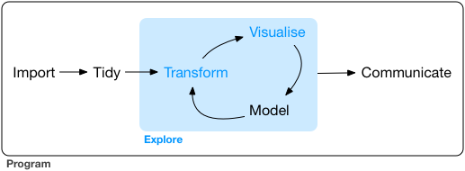
Datenvisualisierung mit ggplot2
Funktionsweise der ggplot Funktion
Leere Leinwand. age auf der x-Achse und days_to_death auf der y-Achse.
ggplot(hnscc, aes(x=age, y=days_to_death))
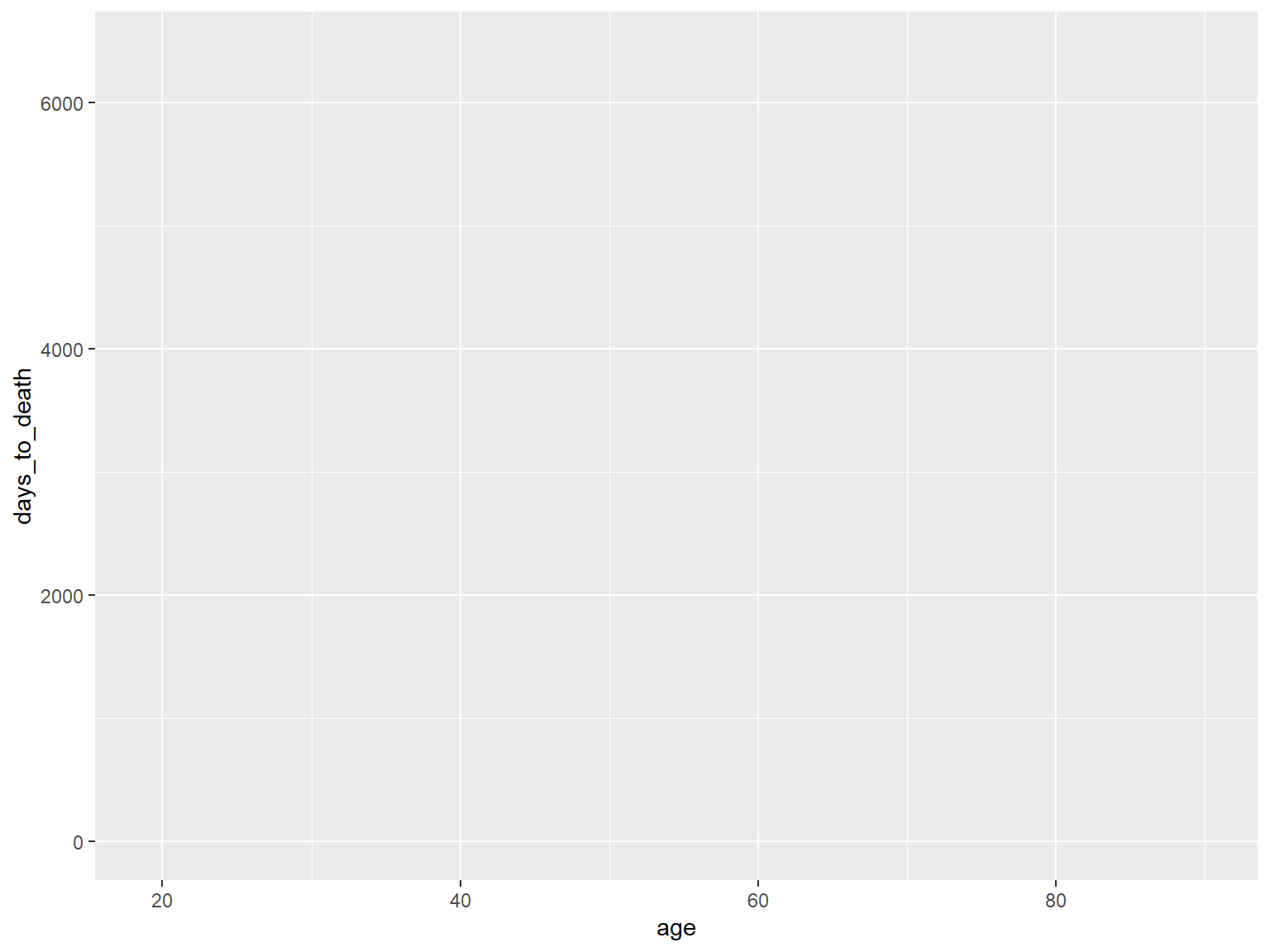
ggplot(hnscc, aes(x=age, y=days_to_death))
Mit den sogenannten Aesthetics aes definieren wir die Dimensionen an Informationen, die wir im Plot darstellen möchten.
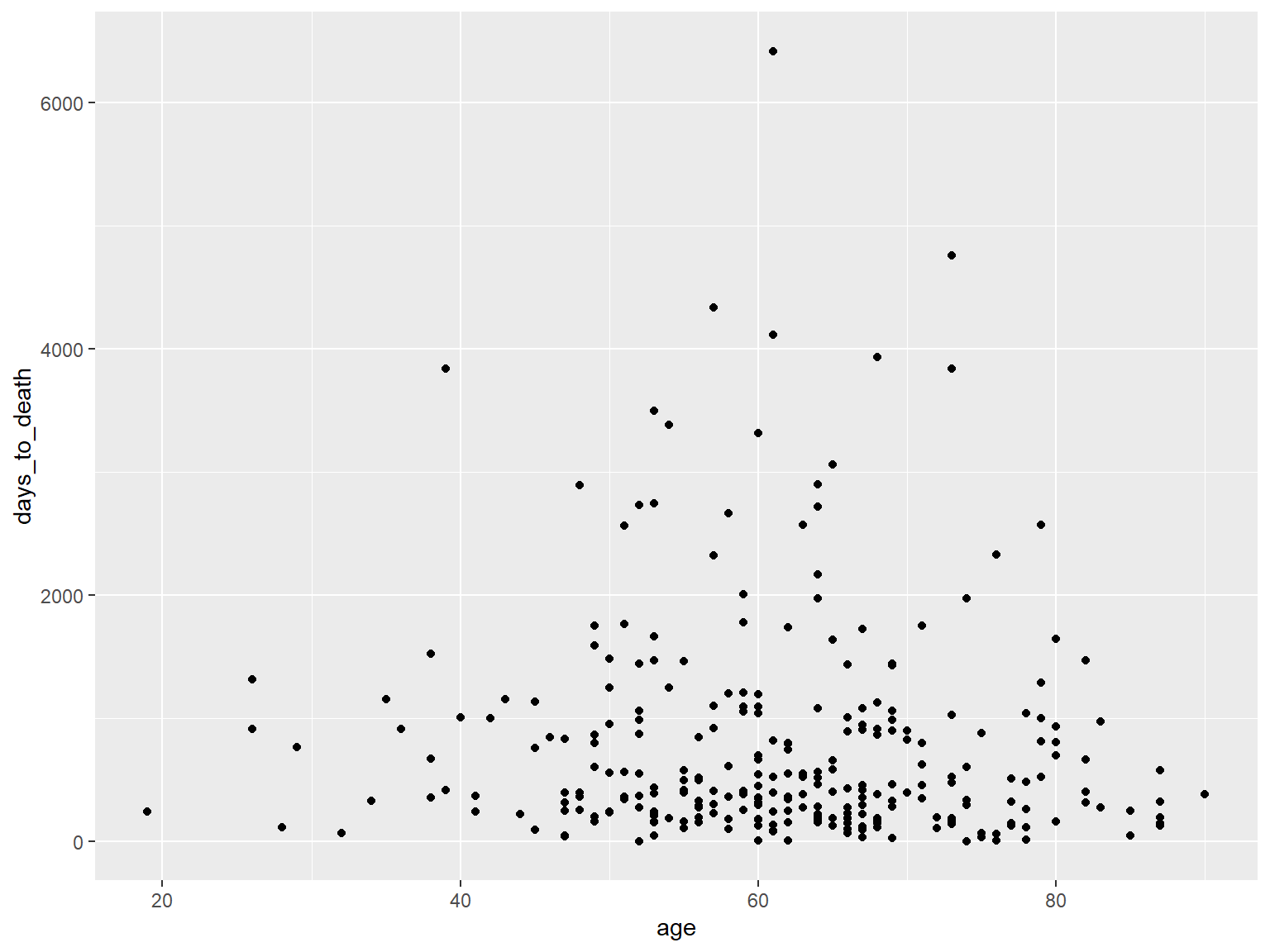
Dieser leeren Leinwand werden nun sogenannte geoms hinzugefügt, z.B. geom_point für einen Dotplot.
ggplot(hnscc, aes(x=age, y=days_to_death)) +
    geom_point()
Dotplot
ggplot(hnscc, aes(x=age, y=days_to_death)) +
    geom_point()
## Warning: Removed 1 rows containing missing values (geom_point).
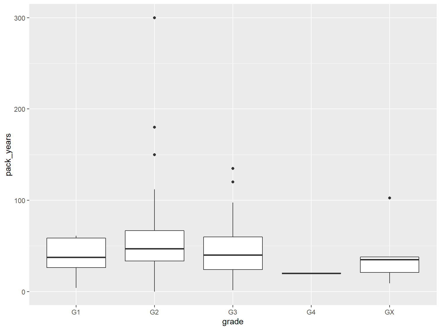
Boxplot
ggplot(hnscc, aes(x=grade, y=pack_years)) +
    geom_boxplot()
## Warning: Removed 125 rows containing non-finite values (stat_boxplot).
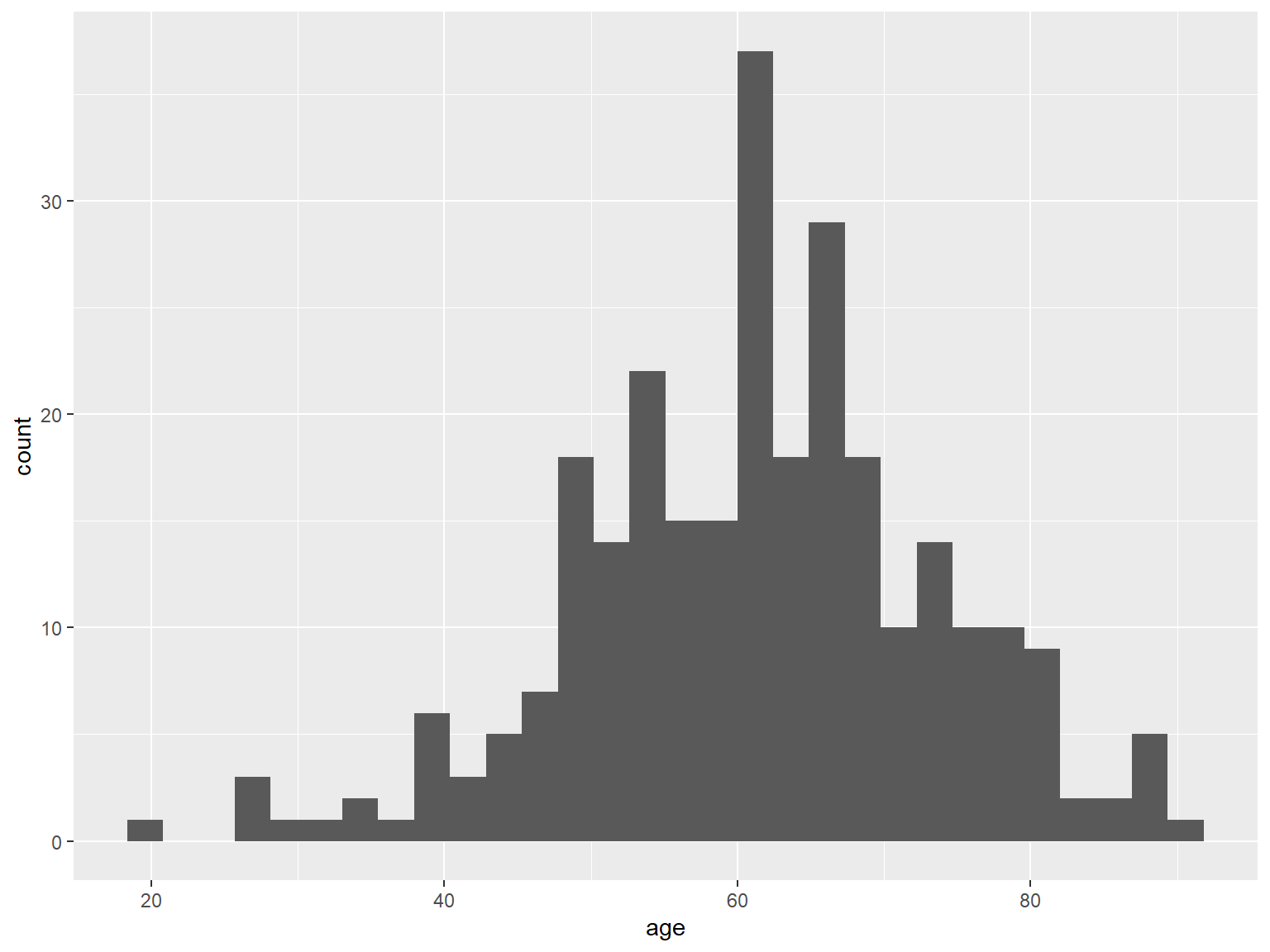
Histogramm
ggplot(hnscc, aes(x=age)) +
    geom_histogram()
## `stat_bin()` using `bins = 30`. Pick better value with `binwidth`.
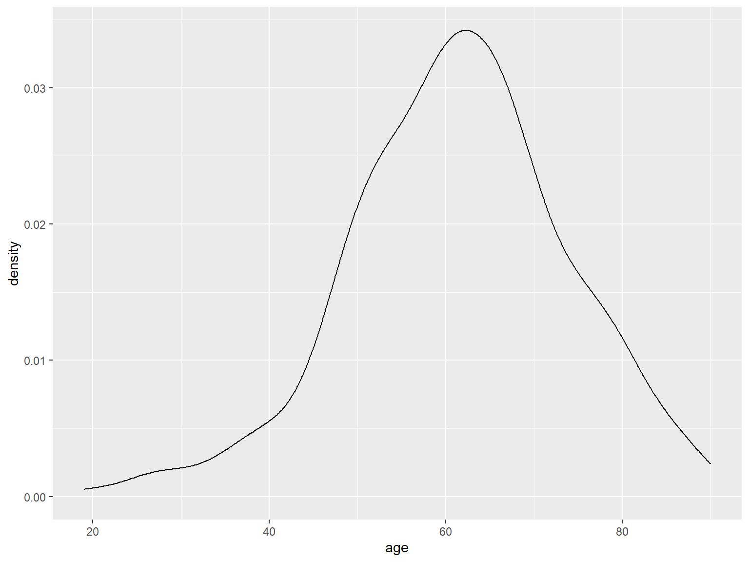
Density plot
ggplot(hnscc, aes(x=age)) +
    geom_density()
Aesthetics
Bisher haben wir als aesthetics nur die x- und y-Achse verwendet. ggplot2 bietet jedoch noch weitere Dimensionen von Daten als aesthetics zu definieren
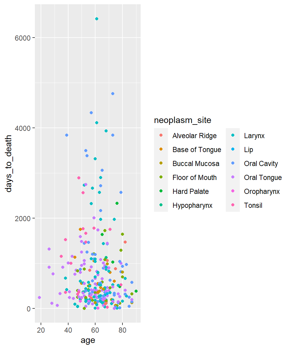
Aesthetic - color
Coloring - kategoriale Variable neoplasm site.
ggplot(hnscc, aes(x=age, y=days_to_death, color=neoplasm_site)) +
    geom_point() +
    guides(color=guide_legend(ncol=2))
## Warning: Removed 1 rows containing missing values (geom_point).
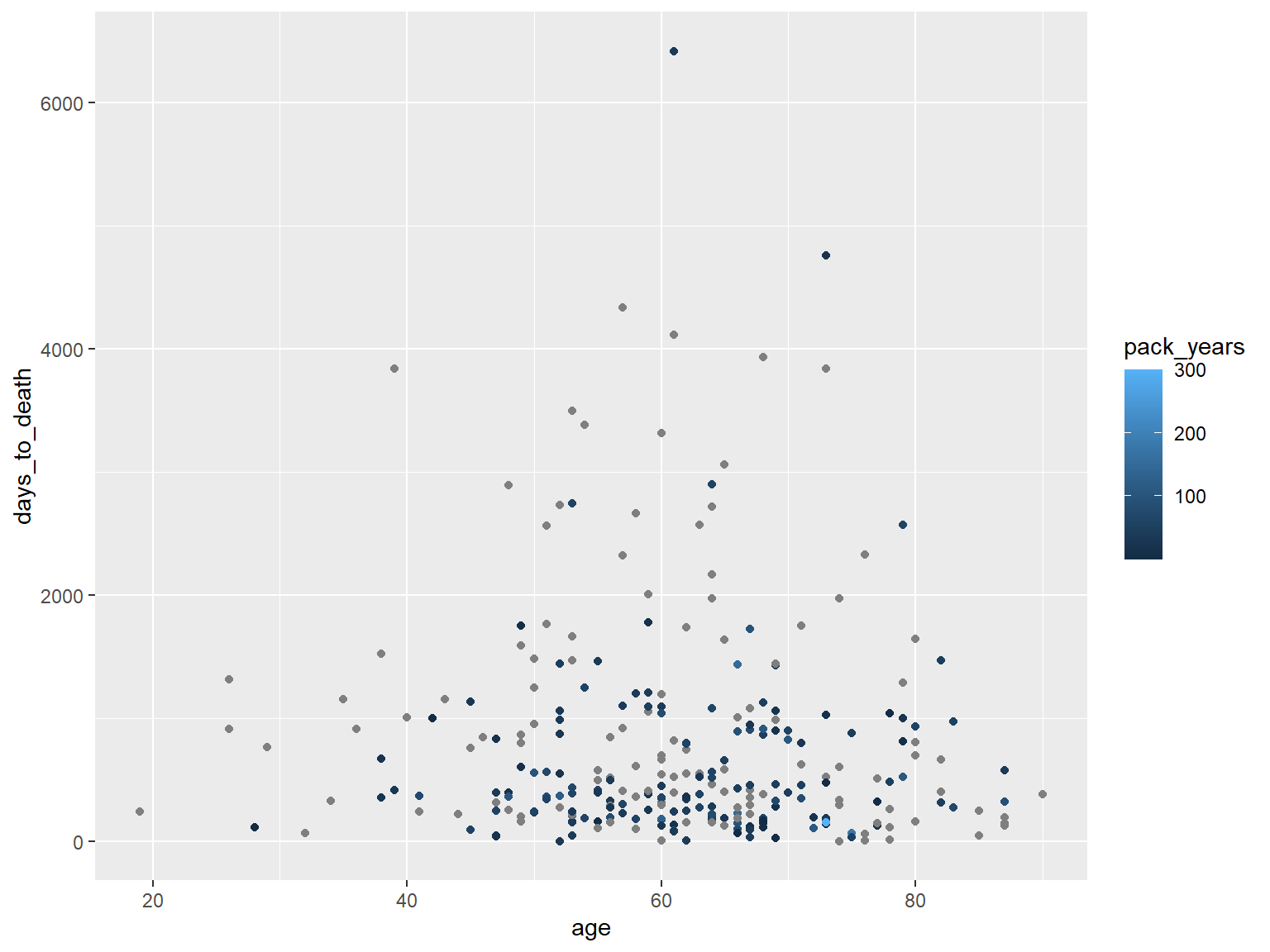
Coloring - numerische Variable packyears.
ggplot(hnscc, aes(x=age, y=days_to_death, color=pack_years)) +
    geom_point()
## Warning: Removed 1 rows containing missing values (geom_point).
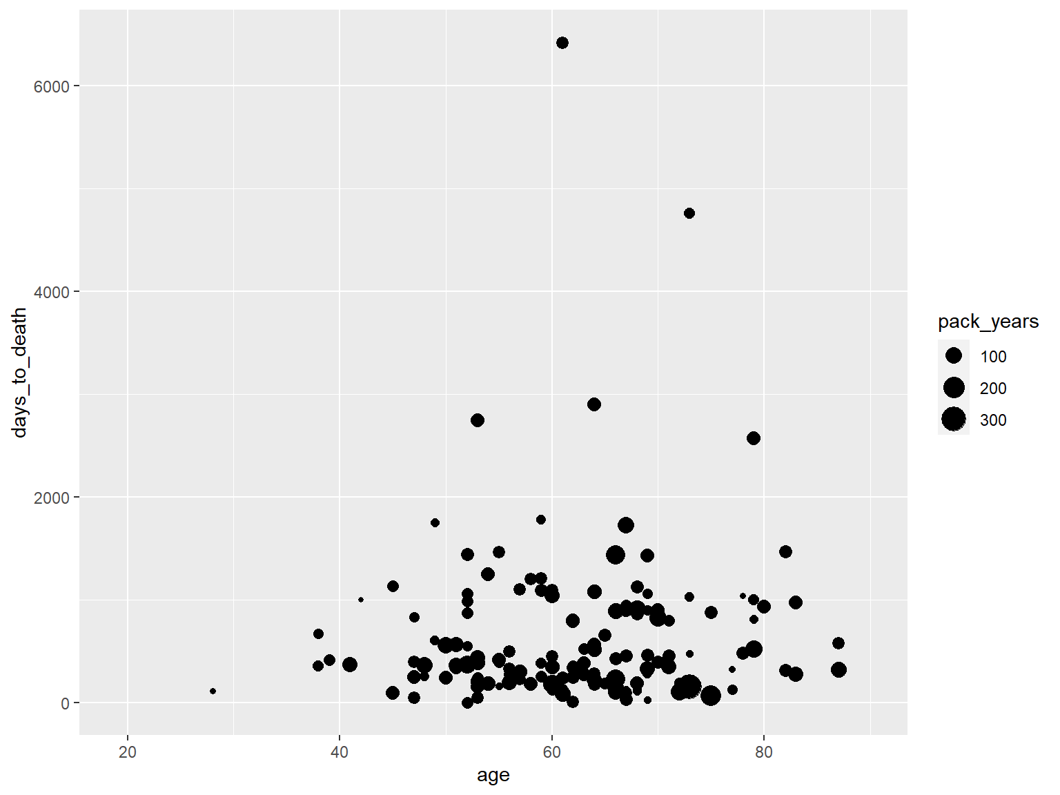
Aesthetic - size
ggplot(hnscc, aes(x=age, y=days_to_death, size=pack_years)) +
    geom_point()
## Warning: Removed 126 rows containing missing values (geom_point).
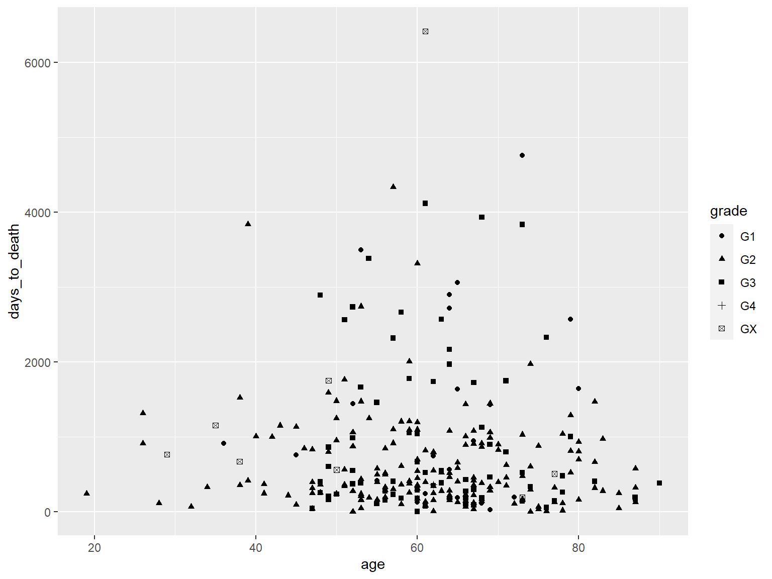
Aesthetic - shape
ggplot(hnscc, aes(x=age, y=days_to_death, shape=grade)) +
    geom_point()
## Warning: Removed 1 rows containing missing values (geom_point).
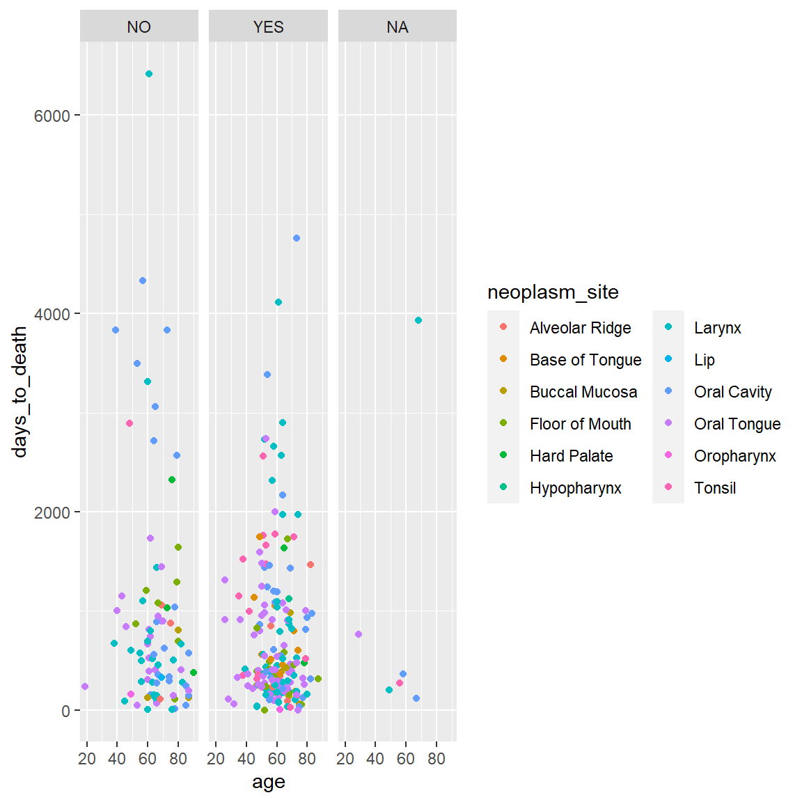
Facetting
Über die Aesthetics hinaus gibt es die Möglichkeit Plots nach kategorialen Variablen zu stratefizieren.
ggplot(hnscc, aes(x=age, y=days_to_death, color=neoplasm_site)) +
    geom_point() +
    facet_wrap(~alcohol) +
    guides(color=guide_legend(ncol=2))
## Warning: Removed 1 rows containing missing values (geom_point).